Operations using pandas
Content of previous tutorial
- Pandas intro
- Series
- DataFrame
- Few operations on Series and DataFrame
Selection:
In the previous tutorial we have learnt , how to select a particular element and subset of the dataframe.
Selecting an element.
DataFrame_name [ ‘row_label’ , ‘col_label’ ]
This would be our data frame for the operations that will be doing in this tutorial, until unless we define some other data frame.
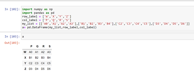
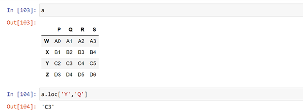
Let us access the element ‘C3’ from this dataframe
It is in ‘Y’ row and ‘Q’ column
a.loc[‘Y’,’Q’] = required element
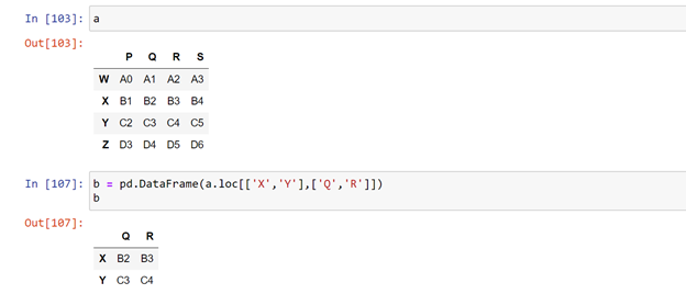
Now let us access a sub set from this data frame and name that dataframe as ‘b’
Conditional Selection:
This is similar to conditional selection, that was explained in numpy tutorials.
Few index operations:
Let us want index to be set to inbuilt values.
Then we have to use a function reset_index ( )
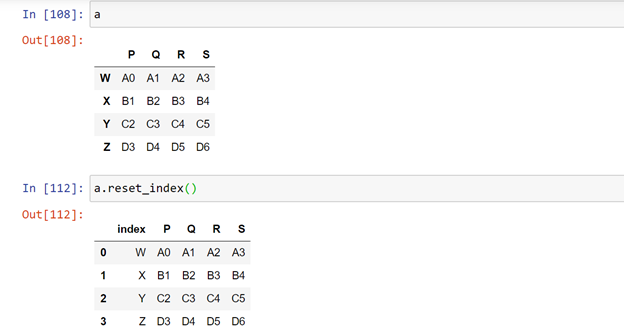
Now if the index should be some of the column , then use set_index ( ) function.
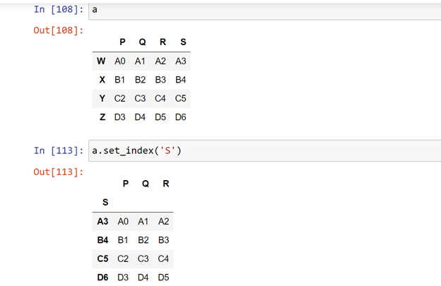
Multi level Indexing:
Sometimes there are multiple columns of indexing, this would be clearly understood using an example. It is also known as hierarchical indexing .
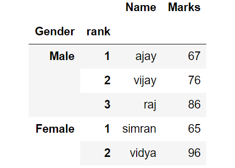
Such form of data is known as multi level indexing , to make such indexing they should have common terms like here Male is common for e members.
In this case multi level indexing was made
df.set_index ( [ ‘Gender’,’rank’ ] )
Pandas on Missing data:
When a huge amount of data is created , there is a probability of getting lot of missing data too. Pandas has ability to find the missing data and replace some suitable form of data.

This is data of few student’s exam marks but some of the marks were not added due to some problem. To check the empty data we pass a function dataFrame.isnull ( )
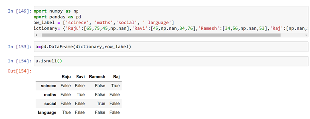
We get Boolean == True where the data was missing. Now we shall either fill the missing values or remove ,to remove the empty box either we have to remove the particular row or particular column.
To remove that row a.dropna( ) # remove row because axis=0 inbuilt
To remove that column a.dropna( axis =1 ) # remove row because axis=1 is meant for column operation
Now let us fill the empty values:
We can fill the empty values using a.fillna( ) function. But here let us fill those empty values with the student average marks.

Instead of writing the code in 2 lines it can be written as

Writing the code as less as much possible would save the memory and will increase the speed. Now let us fill all the missing values.

Keep working with the data, only way to be a good data scientist.
Groupby:
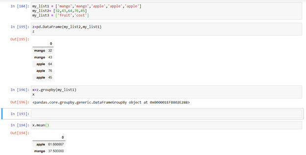
This property allows us to group together data on row basis.

This sort of grouping the data is known as groupby. To do this there should be some common data as above image. Here the logic applied is sum , it could be any other logical operation.
Concatenation:
This function joins two dataframes , condition applied that dimensions should be same along the axis we are joining.
Dataframe_name ( [ df1, df2 ] ) , without any axis argument it is zero .
Here in below example we created three dataframes using numpy random function.
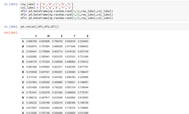
Here the dataframes are concatenated vertically because axis was zero
Now let us try to concatenate horizontally

There is another function by which we can concatenate horizontally without passing the axis parameter as one and that method is transpose( ) , this function is similar we used in matrix, but the labels are interchanged with this method.

